Image Information
The main objectives of this module are:
- Manipulate an image with Python, scikit-image and numpy.
- Process images at the pixel level.
- Compute and understand image histograms.
- Understand lossless compression & reconstruction.
- Understand the co-occurrence matrix.
- Use different colour representations.
1. Read & write an image
In this exercise, we will simply open an image file, display it, and save a copy.
Use the scikit-image io module to open, show & save a copy of the "camera.jpg" image.
Note: we use the %matplotlib inline command to display the image in the notebook. It would not be necessary if you execute the code in the terminal or in a standard IDE like PyCharm.
from skimage.io import imread,imsave,imshow
%matplotlib inline

## -- Your code here -- ##
When you open an image with scikit-image, it is stored as a Numpy ndarray object. Numpy arrays are objects which can be easily manipulated for numerical computations.
Using ndarray methods & attributes, answer the following questions about the "camera" image:
- What is the shape of the image? (width & height)
- What is the minimum pixel value? What is the maximum pixel value?
- What is the data type for each pixel?
- Show only a 100x100 pixels window taken at the center of the image.
import numpy as np

## -- Your code here -- ##
Need more help? You can check the following videos:
2. Image histograms
- Compute and plot the histogram and the normalized histogram of the example cameraman image given below.
You can use the pyplot module from matplotlib to display plots & histograms.
from matplotlib import pyplot as plt

## -- Your code here -- ##
Can you use the histogram to answer the following questions ? (you don't need to code anything here)
- What is the average gray value of the cameraman ?
- What is the average gray value of the sky ?
- Is there more 'cameraman' pixels than 'sky' pixels ?
Compute and plot the cumulated histogram.
## -- Your code here -- ##
Need more help? You can check the following videos:
3. Image entropy
The "entropy" of a signal, in information theory, can generally be interpreted as the "number of bits required to encode the signal". It is a measure of the "amount of information" contained in the signal. Intuitively, a signal with a very narrow distribution (all values are close to each other) will have a very low entropy, while a signal with a wide distribution (the values are evenly distributed) will have a higher entropy.
- Compute the image entropy of the cameraman image. The image entropy is given by $e = - \sum_{g=0}^N p(g) \log_2(p(g))$ where $p(g)$ is the probability that a pixel has the grayscale value g, and N is the number of possible grayscale values. Note that p(g) is directly given by the normalized histogram.
- What is the entropy of a shuffled version of the cameraman ?
# -- Your code here -- #
Need more help? You can check the following videos:
4. Image compression
Using the code below as a starting point:
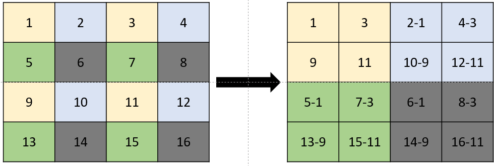
- Decompose an image by recursively subsampling its dimensions and computing the remainders, such that each level of recursion performs the following operation:
%matplotlib inline
import numpy as np
import matplotlib.pyplot as plt
from matplotlib import cm
from skimage.io import imread

# Modify this method:
def split(im):
    a = im[0:-1:2,0:-1:2]
    b = im[0:-1:2,1::2]
    c = im[1::2,0:-1:2]
    d = im[1::2,1::2]

    R = np.vstack((np.hstack((a,b)),np.hstack((c,d))))
    return R

im = imread('camera.jpg').astype(np.int16) # cast the camera image as a signed integer to avoid overflow
s = split(im)

plt.figure(figsize=(12,12))
# interpolation='nearest' -> don't try to interpolate values between pixels if the size of the display is different from the size of the image
# cmap=cm.gray -> display in grayscale
# vmin=-255 -> set "black" as -255
# vmax=255 -> set "white" as 255
plt.imshow(s,interpolation='nearest',cmap=cm.gray,vmin=-255, vmax=255)
plt.colorbar()

plt.show()

Compute how the image entropy evolves with regards to the level of decomposition
# -- Your code here -- #
Rebuild the original image from the pyramid (allowing the selection the level of recursion)
# -- Your code here -- #
Need more help? You can check the following videos:
5. Co-occurrence matrix
While the histogram of an image is independent of the position of the pixels, the co-occurrence matrix gives us information about their spatial distribution.
A co-occurrence matrix is computed for a given displacement, looking at the pair of values spatially separated by that displacement. The co-occurrence matrix is a square matrix, its size given by the number of possible values that a pixels can take in the image.
- Compute de cooccurrence matrix for a chosen displacement $(\Delta x,\Delta y)$ (see greycomatrix in scikit-image)
- What is the entropy of the cooccurrence matrix ?
- How does this entropy evolve if we increase the displacement ?
from skimage.feature import greycomatrix

# -- Your code here -- #
Need more help? You can check the following videos:
6. Colour representations
A colour image is typically encoded with three channels: Red, Green and Blue. In the example below, we open the immunohistochemistry() example image and split it into the three channels, which we display:
from skimage.data import immunohistochemistry

im = immunohistochemistry() # scikit-image method to load the example image
print(im.shape,im.dtype)
r = im[:,:,0]
g = im[:,:,1]
b = im[:,:,2]

plt.gray() # Use grayscale by default on 1-channel images, so you don't have to add cmap=plt.cm.gray everytime

plt.figure(figsize=(12,12))
plt.subplot(2,2,1)
plt.imshow(im)
plt.title('RGB')
plt.subplot(2,2,2)
plt.imshow(r)
plt.title('Red')
plt.subplot(2,2,3)
plt.imshow(g)
plt.title('Green')
plt.subplot(2,2,4)
plt.imshow(b)
plt.title('Blue')
plt.show()
(512, 512, 3) uint8
<Figure size 432x288 with 0 Axes>

- Compute & show the color histograms
- Convert the image to the HSV color space & compute the HSV histograms. See the skimage documentation for reference on color transformation
- Find a method to isolate the brown cells in the immunohistochemistry image
- In the RGB space
- In the HSV space
# -- Your code here -- #
Need more help? You can check the following videos:
Coding Project - Watermark
Write code to automatically add a watermark to a photograph.
Main requirements
The minimum requirements are to:
- Add the white pixels from the watermark somewhere in the photograph.
- Save the resulting image as an image file & display it in the notebook
You may use the watermark.png file available in the GitHub repository, or choose/create your own.
Additional requirements
(note: this is not an exhaustive list, use your imagination!)
- Add an option to choose the watermark location
- Add transparency effect to the watermark
- Determine if the watermark should be dark or light based on the luminosity of the image
- ...
# -- Your code here -- #