Detectors
%matplotlib inline
from skimage import data
import cv2
import matplotlib.pyplot as plt
from matplotlib.patches import Rectangle
import numpy as np
import matplotlib.cm as cm
from scipy import ndimage,interpolate
from scipy.ndimage.filters import convolve1d
Harris corner detection
see also https://docs.opencv.org
Let's look for corners. Since corners represents a variation in the gradient in the image, we will look for this "variation".
ima = np.zeros((50,50),dtype=np.uint8)
ima[20:40,20:30] = 1

def add_rect(ax,xy,c='r',rand=None):
    rect = Rectangle(xy,7,7,facecolor="none", edgecolor=c, alpha=0.8)
    ax.add_patch(rect)
    if rand:
        for i in range(5):
            rxy = (xy[0]+rand*np.random.rand()-rand/2,xy[1]+rand*np.random.rand()-rand/2)
            add_rect(ax,rxy,c='g')

fig, ax = plt.subplots()
plt.imshow(ima)
add_rect(ax,(16,16),rand=3)
add_rect(ax,(4,16))
add_rect(ax,(16,30))
plt.imshow(ima)
plt.show()

Consider a grayscale image $I$. We are going to sweep a window $w(x,y)$ (with displacements u in the x direction and v in the y direction) $I$ and will calculate the variation of intensity.
\begin{equation} E(u,v) = \sum _{x,y} w(x,y)[ I(x+u,y+v) - I(x,y)]^{2} \end{equation}where:
$w(x,y)$ is the window at position $(x,y)$
$I(x,y)$ is the intensity at $(x,y)$
$I(x+u,y+v)$ is the intensity at the moved window $(x+u,y+v)$
Since we are looking for windows with corners, we are looking for windows with a large variation in intensity. Hence, we have to maximize the equation above, specifically the term:
$\sum _{x,y}[ I(x+u,y+v) - I(x,y)]^{2}$
Using Taylor expansion of $I(x+u,y+v)$
\begin{equation} E(u,v) \approx \sum _{x,y} w(x,y) [ I(x,y) + u I_{x} + vI_{y} - I(x,y)]^{2} \end{equation}where $I_{x}$ and $I_{y}$ are x and y image derivatives.
Image derivative
Image derivative can be approximated by discrete differentiation operators
\begin{equation} f'(x) = \lim_{h\to0} \frac{f(x+h) - f(x)}{h} \end{equation}for images, the equivallent is given by the convolution ($*$) of the image $I$ by the Prewitt operator,
\begin{equation} I_x = \begin{bmatrix} +1 & 0 & -1 \\ +1 & 0 & -1 \\ +1 & 0 & -1 \end{bmatrix} * I \end{equation}\begin{equation} \mbox{and} \quad \quad I_y = \begin{bmatrix} +1 & +1 & +1 \\ 0 & 0 & 0 \\ -1 & -1 & -1 \end{bmatrix} * I \end{equation}
that gives:
\begin{equation} E(u,v) \approx \sum _{x,y} w(x,y) (u^{2}I_{x}^{2} + 2uvI_{x}I_{y} + v^{2}I_{y}^{2}) \end{equation}Which can be expressed in a matrix form as:
\begin{equation} E(u,v) \approx \begin{bmatrix} u & v \end{bmatrix} \left ( \displaystyle \sum_{x,y} w(x,y) \begin{bmatrix} I_x^{2} & I_{x}I_{y} \\ I_xI_{y} & I_{y}^{2} \end{bmatrix} \right ) \begin{bmatrix} u \\ v \end{bmatrix} \end{equation}\begin{equation} E(u,v) \approx \begin{bmatrix} u & v \end{bmatrix} M \begin{bmatrix} u \\ v \end{bmatrix} \end{equation}with
\begin{equation} M = \displaystyle \sum_{x,y} w(x,y) \begin{bmatrix} I_x^{2} & I_{x}I_{y} \\ I_xI_{y} & I_{y}^{2} \end{bmatrix} \end{equation}Harris suggested to use the following expression to speed up the corner detection instead of explicitely compute $\lambda_{1,2}$
\begin{equation} R = det(M) - k(trace(M))^{2} \label{eq:vector_ray} \end{equation}where:
$det(M) = \lambda_{1}\lambda_{2}$
$trace(M) = \lambda_{1}+\lambda_{2}$
When $|R|$ is small, which happens when $\lambda_1$ and $\lambda_2$ are small, the region is flat.
When $R<0$, which happens when $\lambda_1 >> \lambda_2$ or vice versa, the region is edge.
When $R$ is large, which happens when $\lambda_1$ and $\lambda_2$ are large and $\lambda_1 \sim \lambda_2$, the region is a corner.
Shi-Tomasi
As an alternative to Harris' $R$, authors suggested to use:
$ R = \min(\lambda_1, \lambda_2) $
see Shi J and Tomasi C (1994). Good Features to Track. In: Proceedings of the IEEE Computer Society Conference on Computer Vision and Pattern Recognition (CVPR), pp 593–600.
Subpixel accuracy
Application to corner detection
from matplotlib import pyplot as plt

from skimage import data
from skimage.feature import corner_harris, corner_subpix, corner_peaks
from skimage.transform import warp, AffineTransform
from skimage.draw import ellipse

# Sheared checkerboard
tform = AffineTransform(scale=(1.3, 1.1), rotation=1, shear=0.7,
                        translation=(110, 30))
image = warp(data.checkerboard()[:90, :90], tform.inverse,
             output_shape=(200, 310))
# Ellipse
rr, cc = ellipse(160, 175, 10, 100)
image[rr, cc] = 1
# Two squares
image[30:80, 200:250] = 1
image[80:130, 250:300] = 1

coords = corner_peaks(corner_harris(image), min_distance=5, threshold_rel=0.02)
coords_subpix = corner_subpix(image, coords, window_size=13)

fig, ax = plt.subplots(figsize=[10,10])
ax.imshow(image, cmap=plt.cm.gray)
ax.plot(coords[:, 1], coords[:, 0], color='cyan', marker='o',
        linestyle='None', markersize=6)
ax.plot(coords_subpix[:, 1], coords_subpix[:, 0], '+r', markersize=15)
ax.axis((0, 310, 200, 0))
plt.show()

Harris corner detection suffers from a major issue, it is not scale invariant, cornerness, especially for a discrete image, depends on the image scale, this problem is taken into account with the two next detectors:
SIFT Scale-Invariant Feature Transform
SURF Speeded Up Robust Features
SIFT (Scale-Invariant Feature Transform)
Lowe, David G. (1999). "Object recognition from local scale-invariant features". Proceedings of the International Conference on Computer Vision. 2. pp. 1150–1157.
maxima and minima of the DoG, Difference of Gaussian, in the scale space
scale space obtained by filtering and sub-sampling
lower contrast points are eliminated (local maximum with 26 neib.)
local orientation signature using the histogram of oriented gradients
image = np.zeros((40,125),dtype=np.uint8)
rr, cc = ellipse(20, 60, 10, 50)
image[rr, cc] = 1
big_image = cv2.resize(image,(image.shape[1]*10,image.shape[0]*10),interpolation=cv2.INTER_NEAREST)

coords = corner_peaks(corner_harris(image), min_distance=5, threshold_rel=0.04)
big_coords = corner_peaks(corner_harris(big_image), min_distance=5, threshold_rel=0.04)


fig, ax = plt.subplots(2,figsize=[10,10])
ax[0].imshow(image, cmap=plt.cm.gray)
ax[0].plot(coords[:, 1], coords[:, 0], color='cyan', marker='o',
        linestyle='None', markersize=6,alpha=.7)
ax[1].imshow(big_image, cmap=plt.cm.gray)
ax[1].plot(big_coords[:, 1], big_coords[:, 0], color='cyan', marker='o',
        linestyle='None', markersize=6,alpha=.7)
plt.show()

Pyramid images
Multi-scale approach using pyramidal image decomposition
from scipy.ndimage.filters import gaussian_filter
from skimage.data import camera
import matplotlib.pyplot as plt
import matplotlib.cm as cm

def build_gaussian_pyramid(ima,levelmax):
    """return a list of subsampled images (using gaussion pre-filter
    """
    r = [ima]
    current = ima
    for level in range(levelmax):
        lp = gaussian_filter(current,1.0)
        sub = lp[::2,::2]
        current = sub
        r.append(current)
    return r

def build_pyramid(ima,levelmax):
    """return a list of subsampled images (using gaussion pre-filter
    """
    r = [ima]
    current = ima
    for level in range(levelmax):
        sub = current[::2,::2]
        current = sub
        r.append(current)
    return r

im = camera()[::2,::2]

#build filtered and non-filtered pyramids
N = 4
fpyramid = build_gaussian_pyramid(im,N)
nfpyramid = build_pyramid(im,N)

fig, ax = plt.subplots(N+1,2,figsize=[10,25])

for i,(f,nf) in enumerate(zip(fpyramid,nfpyramid)):
    ax[i][0].imshow(f,cmap=plt.cm.gray,interpolation='nearest')
    ax[i][0].set_title('guaussian pyramid')
    ax[i][1].imshow(nf,cmap=plt.cm.gray,interpolation='nearest')
    ax[i][1].set_title('subsampling pyramid');

plt.show()

Histogram of oriented gradient (HoG)
In order to differentiate each detected corner, one can compute local descriptors. Local gradient orientation distribution can be used.
Gradient direction can be computed from local image $x$ and $y$ derivatives
\begin{equation} I_x = \begin{bmatrix} +1 & 0 & -1 \\ \end{bmatrix} * \mathbf{I} \end{equation}\begin{equation} \mbox{and} \quad \quad I_y = \begin{bmatrix} +1 \\ 0 \\ -1 \end{bmatrix} * \mathbf{I} \end{equation}then gradient is \begin{align} \nabla I(x, y) = \left(I_x, I_y\right)\\ \end{align}
Amplitude and angle: \begin{align} amplitude &= \sqrt { I_x^2 + I_y^2 }\\ angle &= \tan^{-1}( \frac{I_x}{I_y})\\ \end{align}
def plot_arrows(z,ax,sub=1):

    m,n = z.shape
    x,y = np.meshgrid(range(0,m,sub),range(0,n,sub))
    w = np.array([-1,0,+1])

    dx = convolve1d(z,w,axis=1,origin=0)
    dy = convolve1d(z,w,axis=0,origin=0)

    ax.imshow(z,alpha=.1)
    ax.quiver(x,y,dx[::sub,::sub],dy[::sub,::sub],angles='xy',scale_units='xy', scale=.5, pivot='mid' )


z = ima.astype(np.int8)

fig, ax = plt.subplots()
plot_arrows(z,ax)
plt.show()

z = data.camera()/10.

fig, ax = plt.subplots()
plot_arrows(z,ax,sub=10)
plt.show()

the local distribution of the gradient direction is a good signature to describe a point of interest.
Hereafter the detection of the SIFT corners (position/scale and orientation)
g = data.astronaut()
sift = cv2.SIFT_create()
kp = sift.detect(g,None)
img=cv2.drawKeypoints(g,kp,g,flags=cv2.DRAW_MATCHES_FLAGS_DRAW_RICH_KEYPOINTS)
plt.imsave('astro_points.png',img)
plt.figure()
plt.imshow(img)
plt.show()

SURF (Speeded Up Robust Features)
speed up of the second derivative of the gaussian by using the integral images
Herbert Bay, Andreas Ess, Tinne Tuytelaars, Luc Van Gool, "SURF: Speeded Up Robust Features", Computer Vision and Image Understanding (CVIU), Vol. 110, No. 3, pp. 346--359, 2008
Integral images
In order to speed up computation some approximation can be done. One very intersting algorithm is the integral image.
ima = np.zeros((50,50),dtype=np.uint8)
ima[20:30,20:30] = 1
ima[40:45,10:15] = 1
plt.figure(figsize=[10,10])
plt.subplot(1,2,1)
plt.imshow(ima)
integral_image = cv2.integral(ima)
plt.subplot(1,2,2)
plt.imshow(integral_image,cmap=plt.cm.hot)

from mpl_toolkits.mplot3d import axes3d

fig = plt.figure()
ax = fig.add_subplot(111, projection='3d')

# Grab some test data.
Z = integral_image
m,n = Z.shape
X, Y = np.mgrid[0:m,0:n]

# Plot a basic wireframe.
ax.plot_wireframe(X, Y, Z, rstride=1, cstride=1)


plt.show()


class quad():
    def __init__(self,xy,w,h):
        self.xy = xy
        self.w = w
        self.h = h
        self.pos_a = (xy[1], xy[0])
        self.pos_b = (xy[1] + h, xy[0])
        self.pos_c = (xy[1] + h, xy[0] + w)
        self.pos_d = (xy[1], xy[0] + w)

    def sample(self,image):
        a = image[self.pos_a]
        b = image[self.pos_b]
        c = image[self.pos_c]
        d = image[self.pos_d]
        return a+c-d-b,(a,b,c,d)

    def plot(self,ax,c='r',txt=True):
        rect = Rectangle(self.xy,self.w,self.h,facecolor=c, alpha=0.8)
        ax.add_patch(rect)
        if txt:
            for s,p in zip(['a','b','c','d'],[self.pos_a,self.pos_b,self.pos_c,self.pos_d]):
                ax.text(p[1],p[0],s,c='y')

q = quad((15,15),10,10)

fig, ax = plt.subplots()

plt.imshow(ima)
q.plot(ax)
s,abcd = q.sample(integral_image)
print(f'integral = {s}, abcd = {abcd}')

plt.show()
integral = 25, abcd = (0, 0, 25, 0)

q1 = quad((15,15),4,4)
q2 = quad((15,19),4,4)
q3 = quad((15,23),4,4)

fig, ax = plt.subplots()
plt.imshow(ima)
q1.plot(ax,txt=False)
q2.plot(ax,c='y',txt=False)
q3.plot(ax,txt=False)
s1,_ = q1.sample(integral_image)
s2,_ = q2.sample(integral_image)
print(f's1: {s1}, s2: {s2}')

plt.show()
s1: 0, s2: 0

q1 = quad((5,5),2,2)
q2 = quad((5,7),2,2)
q3 = quad((5,9),2,2)

fig, ax = plt.subplots()
plt.imshow(ima)
q1.plot(ax,txt=False)
q2.plot(ax,c='y',txt=False)
q3.plot(ax,txt=False)
s1,_ = q1.sample(integral_image)
s2,_ = q2.sample(integral_image)
print(f's1: {s1}, s2: {s2}')

plt.show()
s1: 0, s2: 0

q1 = quad((5,5),2,2)
q2 = quad((5,7),2,2)
q3 = quad((7,7),2,2)
q4 = quad((7,5),2,2)

fig, ax = plt.subplots()
plt.imshow(ima)
q1.plot(ax,txt=False)
q2.plot(ax,c='y',txt=False)
q3.plot(ax,txt=False)
q4.plot(ax,c='y',txt=False)

s1,_ = q1.sample(integral_image)
s2,_ = q2.sample(integral_image)
print(f's1: {s1}, s2: {s2}')

plt.show()
s1: 0, s2: 0

FAST
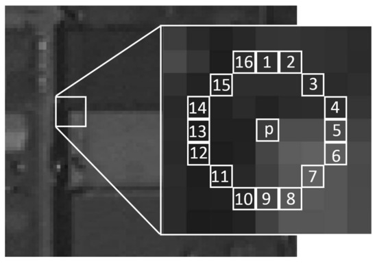
A pixel $p$ is considered as a corner if one of the two folllowing conditions is met:
A set of $N$ contiguous pixels $S$, $\forall x \in S$, the intensity of $x$, $I(x) > I(p) + t$
A set of $N$ contiguous pixels $S$, $\forall x \in S$, $I(x) < I(p) - t$
Rosten, E., and T. Drummond. 2005. “Fusing points and lines for high performance tracking.”P. 1508–1515 in Computer Vision, 2005. ICCV 2005. Tenth IEEE International Conference on, vol. 2. IEEE http://ieeexplore.ieee.org/xpls/ abs_all.jsp?arnumber=1544896 (Accessed February 8, 2011).
Rosten, Edward, and Tom Drummond. 2006. “Machine learning for high-speed corner detection.” Computer Vision–ECCV 2006 430–443. http://www.springerlink.com/index/y11g42n05q626127.pdf (Accessed February 8, 2011).
Application : image warping
from OpenCV examples
import numpy as np
from matplotlib import pyplot as plt

from skimage import data
from skimage.util import img_as_float
from skimage.feature import (corner_harris, corner_subpix, corner_peaks,
                             plot_matches)
from skimage.transform import warp, AffineTransform
from skimage.exposure import rescale_intensity
from skimage.color import rgb2gray
from skimage.measure import ransac


# generate synthetic checkerboard image and add gradient for the later matching
checkerboard = img_as_float(data.checkerboard())
img_orig = np.zeros(list(checkerboard.shape) + [3])
img_orig[..., 0] = checkerboard
gradient_r, gradient_c = (np.mgrid[0:img_orig.shape[0],
                                   0:img_orig.shape[1]]
                          / float(img_orig.shape[0]))
img_orig[..., 1] = gradient_r
img_orig[..., 2] = gradient_c
img_orig = rescale_intensity(img_orig)
img_orig_gray = rgb2gray(img_orig)

# warp synthetic image
tform = AffineTransform(scale=(0.9, 0.9), rotation=0.2, translation=(20, -10))
img_warped = warp(img_orig, tform.inverse, output_shape=(200, 200))
img_warped_gray = rgb2gray(img_warped)

# extract corners using Harris' corner measure
coords_orig = corner_peaks(corner_harris(img_orig_gray), threshold_rel=0.001,
                           min_distance=5)
coords_warped = corner_peaks(corner_harris(img_warped_gray),
                             threshold_rel=0.001, min_distance=5)

# determine sub-pixel corner position
coords_orig_subpix = corner_subpix(img_orig_gray, coords_orig, window_size=9)
coords_warped_subpix = corner_subpix(img_warped_gray, coords_warped,
                                     window_size=9)


def gaussian_weights(window_ext, sigma=1):
    y, x = np.mgrid[-window_ext:window_ext+1, -window_ext:window_ext+1]
    g = np.zeros(y.shape, dtype=np.double)
    g[:] = np.exp(-0.5 * (x**2 / sigma**2 + y**2 / sigma**2))
    g /= 2 * np.pi * sigma * sigma
    return g


def match_corner(coord, window_ext=5):
    r, c = np.round(coord).astype(np.intp)
    window_orig = img_orig[r-window_ext:r+window_ext+1,
                           c-window_ext:c+window_ext+1, :]

    # weight pixels depending on distance to center pixel
    weights = gaussian_weights(window_ext, 3)
    weights = np.dstack((weights, weights, weights))

    # compute sum of squared differences to all corners in warped image
    SSDs = []
    for cr, cc in coords_warped:
        window_warped = img_warped[cr-window_ext:cr+window_ext+1,
                                   cc-window_ext:cc+window_ext+1, :]
        SSD = np.sum(weights * (window_orig - window_warped)**2)
        SSDs.append(SSD)

    # use corner with minimum SSD as correspondence
    min_idx = np.argmin(SSDs)
    return coords_warped_subpix[min_idx]


# find correspondences using simple weighted sum of squared differences
src = []
dst = []
for coord in coords_orig_subpix:
    src.append(coord)
    dst.append(match_corner(coord))
src = np.array(src)
dst = np.array(dst)


# estimate affine transform model using all coordinates
model = AffineTransform()
model.estimate(src, dst)

# robustly estimate affine transform model with RANSAC
model_robust, inliers = ransac((src, dst), AffineTransform, min_samples=3,
                               residual_threshold=2, max_trials=100)
outliers = inliers == False


# compare "true" and estimated transform parameters
print("Ground truth:")
print(f'Scale: ({tform.scale[1]:.4f}, {tform.scale[0]:.4f}), '
      f'Translation: ({tform.translation[1]:.4f}, '
      f'{tform.translation[0]:.4f}), '
      f'Rotation: {-tform.rotation:.4f}')
print("Affine transform:")
print(f'Scale: ({model.scale[0]:.4f}, {model.scale[1]:.4f}), '
      f'Translation: ({model.translation[0]:.4f}, '
      f'{model.translation[1]:.4f}), '
      f'Rotation: {model.rotation:.4f}')
print("RANSAC:")
print(f'Scale: ({model_robust.scale[0]:.4f}, {model_robust.scale[1]:.4f}), '
      f'Translation: ({model_robust.translation[0]:.4f}, '
      f'{model_robust.translation[1]:.4f}), '
      f'Rotation: {model_robust.rotation:.4f}')

# visualize correspondence
fig, ax = plt.subplots(nrows=2, ncols=1,figsize=[10,10])

plt.gray()

inlier_idxs = np.nonzero(inliers)[0]
plot_matches(ax[0], img_orig_gray, img_warped_gray, src, dst,
             np.column_stack((inlier_idxs, inlier_idxs)), matches_color='b')
ax[0].axis('off')
ax[0].set_title('Correct correspondences')

outlier_idxs = np.nonzero(outliers)[0]
plot_matches(ax[1], img_orig_gray, img_warped_gray, src, dst,
             np.column_stack((outlier_idxs, outlier_idxs)), matches_color='r')
ax[1].axis('off')
ax[1].set_title('Faulty correspondences')

plt.show()
Ground truth:
Scale: (0.9000, 0.9000), Translation: (-10.0000, 20.0000), Rotation: -0.2000
Affine transform:
Scale: (0.9015, 0.8913), Translation: (-9.3136, 14.9768), Rotation: -0.1678
RANSAC:
Scale: (0.8999, 0.9001), Translation: (-10.0005, 19.9744), Rotation: -0.1999

demo/webcam